Some Maths for Dobble

Dobble (also known as Spot-It) is an amazing game that’s both fun and mathematically interesting. This is my take on… remembering it some time in the future.

Table of Contents

• Table of Contents
• What’s the Game About?
• How to Design It?
• Mathematical Pointers
• Another Point of View: Projective Planes
• Let’s Start Simple
• Building Projective Planes
  • Points in Homogeneous Coordinates
  • Lines in Homogeneous Coordinates
  • Putting things together
• Finite Fields of Order pⁿ
  • Simple case: \(n = 1\)
  • Field extension case: \(n > 1\)
  • Irreducible Polynomials
• Summing Up
• Credits
• Updates

What’s the Game About?

Dobble provides a set of \(55\) cards, each with exactly \(8\) pictures on it. The cards are round, so that there is no “preferred” way of orienting them; additionally, pictures are printed in random(ish?) orientation and size, again to avoid providing a preferred orientation for the cards.

The one true fact you know about the deck is: whatever pair of cards you take, there is always exactly one picture that is present in both. No more, no less (even though you might have a hard time in finding the matching picture!).

Based on this property, there are some suggestions of rules for several mini-games, all revolving around the ability to quickly spot the matching picture between two cards.

How to Design It?

If each card had \(54\) pictures on it, it would probably be a trivial task to design the full stack of cards: just take all possible pairs of cards and decide a new picture for the pair. This would involve a non-trivial amount of pictures, because all possible pairs are the following:

54 pairs with card A =  #1 and card B = #2..#55
53 pairs with card A =  #2 and card B = #3..#55
...
 1  pair with card A = #54 and card B = #55

for a total number of \((54 + 1) * 54 / 2 = 1485\) pairs/pictures.

Luckily for the players, each card only has exactly \(8\) pictures on it (try to imagine to find the right matching picture out of \(54\) pictures on each card!) but this makes things much more difficult for the designer, because pictures have to be properly reused across cards in order to guarantee the one true fact about the card deck. Here is where maths come to rescue!

Mathematical Pointers

The Dobble deck design can be framed within a much wider set of problems named block design. Well, actually a t-design. Well, actually a Steiner system with parameters \(S(2, 8, 57)\), meaning:

• there are \(57\) different pictures, from which…
• we form cards (blocks) of \(8\) pictures each, with the constraint that…
• any \(2\) pictures are contained in exactly one card (block).

Wait… what? The last constraint is not the one true fact we discussed earlier. As a matter of fact it is, because if the last constraint didn’t hold, then you would have two or more cards sharing more than one picture, which goes against the one true fact.

Are we any closer to doing the design? Well, from my point of view yes and no. We have a lot of stuff that we can read, of course, but nothing really practical.

Another Point of View: Projective Planes

Let’s attack the problem from a different perspective and think about finite projective planes (PP in the following). They are mathematical objects associated to an integer order value \(n\), comprised of primitives called points and lines (collections of points):

• any two points belong to exactly one line
• any two lines intersect at exactly one point, meaning that have exactly one point in common
• there are exactly \(n + 1\) lines intersecting at any point
• there are exactly \(n + 1\) points belonging to any line

You might spot that there is a duality in the properties above: try to swap line for point and belongs to with intersect at and you basically have the same properties again!

Another property of a PP of order \(n\) is that it contains exactly:

points and the same amount of lines (thanks to the duality above).

Of course Steiner systems and Projective Planes are old friends, because a PP of order \(n\) is “just” a Steiner system \(S(2, n+1, n^2 + n + 1)\), thus implying for Dobble that:

going back to what we said earlier: Dobble is a Steiner system \(S(2, 8, 57)\). It’s also interesting to note that Dobble is actually missing two possible cards.

Why involve PPs anyway? Well… for me it’s a bit easier to understand and explain, that’s it.

Let’s Start Simple

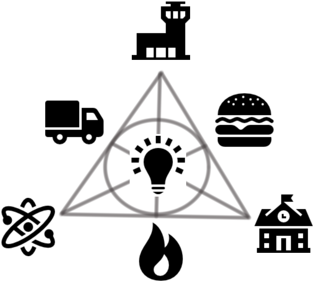
There is one “bare bones” Projective Plane called the Fano Plane, that is of order \(n = 2\). It’s like a stripped down version of Dobble, with “just” \(7 = 4 + 2 + 1\) pictures and (at most) \(7\) cards. A graphical representation of the Fano Plane is in the following picture:

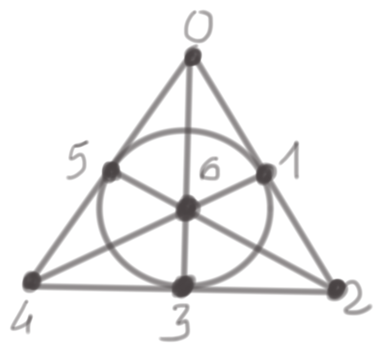
With a leap of imagination, each “bullet” is a point/picture, each segment and the circle is a line/card and there we are:

So, indeed projective planes can be useful for the design task we want to address! We just have to expand things a bit…

Building Projective Planes

The current knowledge about projective planes is more or less the following:

• orders \(n = p^k\), where \(p\) is a prime number and \(k\) is any positive integer are always possible;
• anything else is conjectured to be impossible.

We will restrict to what we know and call “allowed” only orders that are a positive power of a prime number, like in the first bullet.

The Dobble’s case is \(n = 7^1\) so it’s definitely possible, yielding \(57\) pictures and \(57\) cards (of which only 55 are included in the game’s deck, as anticipated).

The logical steps for building a design of any allowed order are the following:

• build a convenient representation of all points
• collect points in lines, leveraging the representation above

It turns out that there is indeed a convenient representation for points that will eventually make it very easy to build lines… so let’s look at it.

Points in Homogeneous Coordinates

Points in a plane are usually represented with two Cartesian coordinates: \(x\) and \(y\). This representation goes under the general name of affine plane. In this plane, it is impossible to represent the point where two or more parallel lines intersect (the “point at infinite”). Additionally, it is also impossible to represent the line formed by all such intersections for different directions, i.e. the “line at infinite”.

As we saw, projective planes require that every pair of lines intersect exactly at one point. Hence, we need a more powerful representation that allows us to easily manipulate these “points at infinite” and the resulting line.

At the expense of one additional coordinate it is indeed possible to represent also these additional points and the additional line, in a system that is called homogeneous coordinates where each point is represented by three coordinates \((X, Y, Z)\) ruled as follows:

• any of \(X\), \(Y\) and \(Z\) MUST be different from \(0\), i.e. the triplet \((0, 0, 0)\) is NOT valid
• a (finite) point \((x, y)\) in the Cartesian representation of the affine plane is mapped onto any triplet \((Z\cdot x, Z\cdot y, Z)\) with \(Z \ne 0\). Conversely, any triplet \((X, Y, Z)\) with \(Z \ne 0\) maps back to \((X/Z, Y/Z)\);
• any triplet \((X, Y, 0)\) is a “point at infinite” and represents the intersection of all parallel lines of type \(Y\cdot x - X\cdot y = c\).

The interesting thing is that we are not necessarily restricted to using real numbers for coordinates: any field will do, including finite fields. (Why fields, anyway? We need the division operation by non-zero to be valid, so fieds are a very useful choice). Let’s take ((Z_2\) for example, i.e. the field whose two elements are the rest classes in the integer division by \(2\): 0 and 1. It’s easy to build up all possible triplets, actually as easy as counting in binary:

0 0 0 <- ruled out, invalid triplet in the homogeneous representation
0 0 1 <- "origin", maps to (0, 0) in the affine plane
0 1 0 <- point at infinite
0 1 1 <- "regular", maps to (0, 1) in the affine plane
1 0 0 <- point at infinite
1 0 1 <- "regular", maps to (1, 0) in the affine plane
1 1 0 <- point at infinite
1 1 1 <- "regular", maps to (1, 1) in the affine plane

There is a total of n^3 - 1 possible points, i.e. 7 in our case. Does this ring a bell? Sure it does, it’s the same number of points in the Fano plane!

Things can get trickier with finite fields of higher orders though, as we can see in the following example in \(Z_3\). We have to remember that homogeneous coordinates with different components might map back to the same point in the affine plane, so we have to only consider the classes of different coordinates and avoid duplicates that can be obtained by scaling already considered ones:

0 0 0 <- ruled out, invalid homogeneous triplet
0 0 1
0 0 2 <- ruled out, (0 0 1) * 2 
0 1 0
0 1 1
0 1 2
0 2 0 <- ruled out, (0 1 0) * 2
0 2 1 <- ruled out, (0 1 2) * 2
0 2 2 <- ruled out, (0 1 1) * 2
1 0 0
1 0 1
1 0 2
1 1 0
1 1 1
1 1 2
1 2 0
1 2 1
1 2 2
2 0 0 <- ruled out, (1 0 0) * 2
2 0 1 <- ruled out, (1 0 2) * 2
2 0 2 <- ruled out, (1 0 1) * 2
2 1 0 <- ruled out, (1 2 0) * 2
2 1 1 <- ruled out, (1 2 2) * 2
2 1 2 <- ruled out, (1 2 1) * 2
2 2 0 <- ruled out, (1 1 0) * 2
2 2 1 <- ruled out, (1 1 2) * 2
2 2 2 <- ruled out, (1 1 1) * 2

Out of the initial \(3^3 = 27\) candidates, only \(13\) survived, so it’s actually a bit more difficult than to simply count and remove the first triplet. Note that this is exactly the number of points we were expecting, because of the formula we saw before: \(3^2 + 3 + 1 = 13\). The distinct points are the following in homogeneous coordinates:

0.  0 0 1
1.  0 1 0
2.  0 1 1
3.  0 1 2
4.  1 0 0
5.  1 0 1
6.  1 0 2
7.  1 1 0
8.  1 1 1
9.  1 1 2
10. 1 2 0
11. 1 2 1
12. 1 2 2

It turns out that there is a simple algoritm for generating all “distinct” homogeneous triplets: just start counting and jump all elements whose leftmost non-\(0\) element is different from \(1\).

Lines in Homogeneous Coordinates

The same reasoning done for points can be repeated for lines. The generic line in the affine plane can be expressed with the following equation:

This equation can be easily multiplied by any non-zero constant, so assuming that \(Z\) is different from \(0\) and remembering the relations of \(x\) with \(X\) and \(y\) with \(Y\):

Hence, a line can be expressed by three values \(a\), \(b\) and \(c\), with the usual rule that any of the three MUST be different from zero. As a matter of fact, it’s yet another place where we see duality at work, because the equation might see the roles of a line’s parameter swapped with the point’s parameters without change in its meaning.

It’s interesting how the equation for a line shows how to find points belonging to the line: it suffices to find all triples \(((X, Y, Z)\) that are “orthogonal” to the line’s triple \((a, b, c)\). Then, by duality, we can also immediately find all lines through a point… because it’s the same equation!

Let’s see what happens with the example based on \(Z_2\):

Line   Homog.   Points in Line (homogen.     Point
Id     repr.    representation)              Ids
0   -> 0 0 1 -> (1 0 0), (0 1 0), (1 1 0) -> 3, 1, 5
1   -> 0 1 0 -> (1 0 0), (0 0 1), (1 0 1) -> 3, 0, 4
2   -> 0 1 1 -> (1 0 0), (0 1 1), (1 1 1) -> 3, 2, 6
3   -> 1 0 0 -> (0 0 1), (0 1 0), (0 1 1) -> 0, 1, 2
4   -> 1 0 1 -> (0 1 0), (1 0 1), (1 1 1) -> 1, 4, 6
5   -> 1 1 0 -> (0 0 1), (1 1 0), (1 1 1) -> 0, 5, 6
6   -> 1 1 1 -> (1 1 0), (1 0 1), (0 1 1) -> 5, 4, 2

We can do the same for \(Z_3\) of course:

Line                                                  Point Ids
Id
 0  -> 0 0 1 -> (1 0 0), (0 1 0), (1 1 0), (1 2 0) -> 4, 1, 7, 10
 1  -> 0 1 0 -> (0 0 1), (1 0 0), (1 0 1), (1 0 2) -> 0, 4, 5, 6
 2  -> 0 1 1 -> (1 0 0), (0 1 2), (1 1 2), (1 2 1) -> 4, 3, 9, 11
 3  -> 0 1 2 -> (1 0 0), (0 1 1), (1 1 1), (1 2 2) -> 4, 2, 8, 12
 4  -> 1 0 0 -> (0 0 1), (0 1 0), (0 1 1), (0 1 2) -> 0, 1, 2, 3
 5  -> 1 0 1 -> (0 1 0), (1 0 2), (1 1 2), (1 2 2) -> 1, 6, 9, 12
 6  -> 1 0 2 -> (0 1 0), (1 0 1), (1 1 1), (1 2 1) -> 1, 5, 8, 11
 7  -> 1 1 0 -> (0 0 1), (1 2 0), (1 2 1), (1 2 2) -> 0, 10, 11, 12
 8  -> 1 1 1 -> (0 1 2), (1 0 2), (1 2 0), (1 1 1) -> 3, 6, 10, 8
 9  -> 1 1 2 -> (0 1 1), (1 0 1), (1 1 2), (1 2 0) -> 2, 5, 9, 10
10  -> 1 2 0 -> (1 1 0), (1 1 1), (1 1 2), (0 0 1) -> 7, 8, 9, 0
11  -> 1 2 1 -> (0 1 1), (1 0 2), (1 1 0), (1 2 1) -> 2, 6, 7, 11
12  -> 1 2 2 -> (0 1 2), (1 0 1), (1 1 0), (1 2 2) -> 3, 5, 7, 12

Putting things together

So, now we have a complete algorithm for finding out projective planes of any “allowed” order:

• build a field of that order. This field always exists:
  • if the order is a prime number \(p\), then the field is simply \(Z_p\), i.e. the field of rest classes modulo \(p\);
  • otherwise, it can be build as a Galois Extension. More on this later, stay tuned!

• find all distinct triplets of homogeneous coordinates. This can be done with the trick of “first non-zero element must be 1” saw before

• for each triplet, find all triplets that are “orthogonal” to it. For example, if the starting triplet is \((X, Y, Z)\), find all triplets \((a, b, c)\) that satisfy the following equation:

• associate an identifier to each triplet, and output the identifier of each one together with the identifiers of the triplets orthogonal to that one.

As an example in Perl, we will use Math::GF for building the field and get all elements inside:

use Math::GF;
my $order = shift // 2;
my @elements = Math::GF->new($order)->all;

We can then proceed to build all distinct triplets representing points, using “the trick” and avoiding the all-zeros triplet:

my $zero = $elements[0];
my $one  = $elements[1];
my @points;
for my $i ($zero, $one) {
   for my $j ($i == $zero ? ($zero, $one) : @elements) {
      for my $k ((($i == $zero) && ($j == $zero)) ? $one : @elements) {
         push @points, [$i, $j, $k];
      }
   }
}

Confused? Take a closer look and you will see that this is exactly the coding of our “trick”:

• the left-most coordinate can only be zero or one, otherwise we would violate the trick
• the mid coordinate can only be zero or one if the previous coordinate is zero, otherwise, again, we would violate the trick. On the other hand, if the previous coordinate is not zero then it will be a one, so it’s OK to consider all elements in the field
• the right-most coordinate MUST be one if the previous ones are both zero, because the triple \((0, 0, 0)\) is not valid in homogeneous coordinates. Otherwise, any element in the field will do.

This formulation also allows us to calculate how many points we will generate. Assuming that there are \(n\) elements in the field:

• \(1\) for \((0, 0, 1)\)
• \(n\) for \((0, 1, k)\) (\(k\) from \(0\) to \(n - 1\))
• \(n^2\) for \((1, j, k)\) (both \(j\) and \(k\) from \(0\) to \(n - 1)\)

which is, again, the formula we saw earlier: \(n^2 + n + 1\).

Now we are ready to build lines by finding orthogonal triplets. We leverage on the same triplets as we found in @points because of duality:

my @lines = map { [] } 1 .. scalar(@points);
for my $li (0 .. $#points) {
   my $L = $points[$li];
   for my $pi ($li .. $#points) {
      last if scalar(@{$lines[$li]}) == $order + 1;
      my $sum = $zero;
      $sum = $sum + $L->[$_] * $points[$pi][$_] for 0 .. 2;
      next if $sum != $zero;
      push @{$lines[$li]}, $pi;
      push @{$lines[$pi]}, $li if $pi != $li;
   }
}

Now @lines is an array of arrays, each containing identifiers of the points belonging to the line. We can easily print them:

sub print_aoa {
   my $aoa = shift;
   printf {*STDOUT} "%3d. (%s)\n", $_, join ', ', @{$aoa->[$_]}
     for 0 .. $#$aoa;
}
print_aoa(\@lines);

The full script can be found here. Sample run with order \(2\):

0. (1, 3, 5)
1. (0, 3, 4)
2. (2, 3, 6)
3. (0, 1, 2)
4. (1, 4, 6)
5. (0, 5, 6)
6. (2, 4, 5)

How to use it for a deck of cards in the game? Simple:

• take your \(n^2 + n + 1\) (7 in the example) blank cards and line them up in front of view. The left-most will be at index 0, then 1, 2, and so on
• take your \(n^2 + n + 1\) (7 in the example) pictures and do the same, again each will get an integer identifier
• read the output of the script in either of the following ways:
  • Fill card 0 with images 1, 3 and 5, or
  • Draw image 0 onto cards 1, 3 and 5

Finite Fields of Order pⁿ

One last bit that was left out from the previous section is building a finite field of a specific order. It turns out that such fields only exist for orders \(p^n\), with \(p\) prime and \(n\) positive integer (e.g. see here).

Simple case: \(n = 1\)

In case \(n = 1\), the field can be simply \(Z_p\), i.e. the field of all rest classes modulo \(p\), under the “usual” sum and multiplication of such rest classes:

• sum: take the sum, then calculate the rest modulo \(p\)
• multiplicaiton: take the product, then calculate the rest modulo \(p\)

With \(p\) prime, the set of rest classes and the operations above will give you a field. For Dobble this would be sufficient because its order - 7 - is indeed a prime number.

Field extension case: \(n > 1\)

What if we want a slightly more difficult variant, e.g. of order 4 (which is \(2^2\), so it’s “allowed”)? Rest classes will not help us in this case because the set of rest classes and the operations above do not form a field (e.g. in \(Z_4\), class \(2_4\) multiplied by itself yields \(0_4\), so it is a divisor of zero which is not allowed in a field).

What we can build in this case is a so-called field extension. The idea is to leverage the field resulting from \(Z_p\) to build an extension over it that accounts for its power \(n\). The intuition to do this is both mindbending and ingenuous.

What is a field? It is a set of elements with two operations defined over those elements, an addition and a multiplication, that have some constraints:

• the set and the addition form a commutative group
• the set without a zero element and the multiplication form a commutative group
• other properties related to distribution, existence of inverse, etc. etc.

With a field, we can build vector spaces, which is a set of elements (vectors) with an operation of addition defined that makes the set a commutative group, plus other stuff involving the field.

The main intuition about field extension is: what if we start from a vector space to build a new field? If you think about it, you’re more than halfway, because you already have a set and an addition operation, so you only need the right multiplication operation and you’re done!

We will gloss over the theoretical details (which can be found in a lot of places around, e.g. here or in the excellent courses by Mattew Salomone) and avoid spoilering too much about a story involving polynomials, multiplications and divisions by irreducible polynomials, to go directly to what we need to do to build a finite field of order \(p^n\):

• start from field \(Z_p\)
• generate all polynomials of degree up to \(n - 1\) over that field, assign an identifier to each of them
• generate the additive table for the extension field like this:

idA -> polyA
idB -> polyB

             +---- sum of polynomials
             v
       polyA + polyB = polyC
       
idC <- polyC

=> idA "+" idB = idC

• generate the multiplicative table. This a bit trickier because the degree of the resulting polynomial might go well beyond the allowed value. This is where the irreducible polynomial gets into play, together with finding the rest in the division by it:

  • find an irreducible polynomial of degree \(n\) over that field (more on this later)

  • generate the multiplicative table like this:

idA -> polyA
idB -> polyB

             +---- multiplication of polynomials
             v
       polyA * polyB = product

               +---- rest operation modulo...
               v
       product % irreducible = polyC
       
idC <- polyC

=> idA "*" idB = idC

As an example, let’s generate GF(4), i.e. the extension of degree 2 of \(Z_2\):

• field: \(Z_2\), elements are 0 and 1
• all polynomials of degree up to \(2 - 1 = 1\):

Id   Polynomial
0    0
1    1
2    x
3    1 + x

• additive table (symmetric, also remember that operations are done modulo 2, so \(1 + 1 = 0\)):

Ids           Polynomials             Id
(0 "+" 0) --> (0 + 0) = 0         --> 0
(0 "+" 1) --> (0 + 1) = 1         --> 1
(0 "+" 2) --> (0 + x) = x         --> 2
(0 "+" 3) --> (0 + 1 + x) = 1 + x --> 3

(1 "+" 1) --> (1 + 1) = 0         --> 0
(1 "+" 2) --> (1 + x) = 1 + x     --> 3
(1 "+" 3) --> (1 + 1 + x) = x     --> 2

(2 "+" 2) --> (x + x) = 0         --> 0
(2 "+" 3) --> (x + 1 + x) = 1     --> 1

(3 "+" 3) --> (1 + x + 1 + x) = 0 --> 0

• irreducible polynomials of degree 2:
  • \(x^2\) is not irreducible because it can be divided by \(x\)
  • \(x^2 + 1\) is not irreducible because it can be divided by \(x + 1\)
  • \(x^2 + x\) is not irreducible because it can be divided by \(x\)
  • \(x^2 + x + 1\) is irreducible, OK!
• multiplicative table (symmetric):

Ids           Polynomials                                 Id
(0 "*" 0) --> (0 * 0) % (x^2 + x + 1) = 0             --> 0
(0 "*" 1) --> (0 * 1) % (x^2 + x + 1) = 0             --> 0
(0 "*" 2) --> (0 * x) % (x^2 + x + 1) = 0             --> 0
(0 "*" 3) --> (0 * (1 + x)) % (x^2 + x + 1) = 0       --> 0

(1 "*" 1) --> (1 * 1) % (x^2 + x + 1) = 1             --> 1
(1 "*" 2) --> (1 * x) % (x^2 + x + 1) = x             --> 2
(1 "*" 3) --> (1 * (1 + x)) % (x^2 + x + 1) = 1 + x   --> 3

(2 "*" 2) --> (x * x) % (x^2 + x + 1) = 1 + x         --> 3
(2 "*" 3) --> (x * (1 + x)) % (x^2 + x + 1) = 1       --> 1

(3 "*" 3) --> ((1 + x) * (1 + x)) % (x^2 + x + 1) = x --> 2

Summarizing, our finite field of \(4\) elements is the following:

elements (identifiers): {0, 1, 2, 3}

 "+"| 0 1 2 3     "*"| 0 1 2 3
 ---+--------     ---+--------
  0 | 0 1 2 3      0 | 0 0 0 0
  1 | 1 0 3 2      1 | 0 1 2 3
  2 | 2 3 0 1      2 | 0 2 3 1
  3 | 3 2 1 0      3 | 0 3 1 2

Irreducible Polynomials

The last thing we might want is some way to find irreducible polynomials of a given degree. To do this, we can iterate over polynomials of that degree and check whether they are irreducible or not, e.g. by means of Rabin’s irreducibility test. You can see some example code in Perl here - this is actually what Math::GF uses internally to generate Galois Fields of non-prime order.

Simpler than this, you can look at some lists available in Internet (e.g. here)!

Summing Up

It’s easy to start from a seemengly innocent game like Dobble and get dragged in some serious maths! The journey was funny although not really linear, which is why I collected these notes and took the time (quite a few) for writing a Perl module for building finite fields!

There is a lot to read around, where you will find exact definitions, demonstration and much better language than you found here. If anything, I can suggest looking at the excellent lessons by Matthew Salomone on YouTube.

Have fun!

Credits

The icons used in the example on the Fano plane are from iconmonstr.

Updates

• 2018-01-08 Cosmetics, better detail how to use output from script
• 2019-09-18 Turn most equations to MathJax-rendered equations